Activity 3: Silhouette Extraction

Did you know that your gait or the way you walk, like your fingerprint, is unique to every individual? What's more interesting is that it can also be analyzed through pattern recognition techniques. In fact, studies conducted on individuals' unique manner of walking, paved the way for experiments on silhouette extraction.

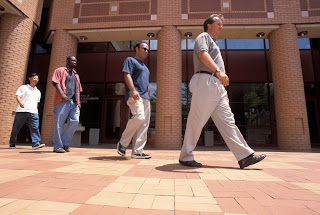
Figure 1. Gait

The study on the gait processing of an individual was initiated in the field of medicine to examine the walking patterns of impaired patients [1,2]. A decade after, it was first used as a pattern recognition technique by Johansson when he used reflectors affixed to the joints of a human body and showed motion sequences as the person walks[3]. The observers were able to identify gender and in some cases person recognition was obtained. Previous works on the use of gait for person identification have mostly utilized side-view gait (pendulum analogy) for feature extraction because temporal variations are more obvious from the side than the front. In this activity, we show and test the biometric feature developed by Soriano et al. that uses the idea of silhouette extraction, the freeman vector code and vector gradients to characterize the concavities and convexities in an image[4].

Experiment

Our first task was to capture an object against a steady background. In one of our conversations in class, Dr. Soriano suggested to use my mouth as the object mainly because she was curious if silhouette extraction can be applied to investigate the relationship between the opening of the mouth and the words (or sound) produced. If we are able to establish the said technique, then it could be a big help in the communication industry since communications with the use of web cameras nowadays is becoming widespread.

We then got the edge of the object of interest using edge detection algorithms and made sure that the edges were one-pixel thick. This is very important as problems may arise in the reconstruction of the curve spreads when the edges are more than a pixel thick. In fact, I encountered problems in the early part of the activity mainly because of the large size of my image and the edges, which were thicker than a pixel. To find the x-y coordinates of the edge, we used the regionprops and pixellist in Matlab.

Figure 2. Sample mouth image (image size: 170 x 122)

Figure 3. Image after applying the edge detection algorithms which include: (a). im2bw (b) edge and bwmorph and imfill.

Note that all the neighboring pixels of an edge pixel can be represented by one number only (from 1 to 8) in the Freeman vector code as shown in Figure 4. We then replaced the edge pixel coordinates with their Freeman Vector Code, took the difference between the codes of two adjacent pixels and performed a running sum of three adjacent gradients. The vector gradient details include: concavity (negative values), convexity (positive numbers bounded by zeros) details and straight line (zeros).

Figure 4. Freeman Vector Code illustration.

Figure 5. The pixel edges of the image with corresponding Freeman Vector code. Inset shows the whole Freeman vector code for the mouth image.

Figure 6. Processed image with corresponding values for the vector gradients. Inset shows the vector gradients for the mouth image.

Figure 6 shows the chain of zeros, positive and negative numbers placed in their appropriate pixel coordinates where zeros are regions of straight lines, negatives are regions of concavities and positives are regions of convexities.

Tips:

One of the more challenging steps in this activity is obtaining an image which is one-pixel thick after edge detection. Before my mouth, which was a success, I tried taking a picture of a hat, a watch and even my pen to no avail.

Since we were able to accurately reconstruct the different regions in the image, this activity may jumpstart the research in identifying the relationship between the shape of the mouth opening and the sound produced. I give myself a grade of 10 in this activity since I was able to reconstruct the regions of straight lines(zeros), concavities(negatives) and convexities(positives) placed in the appropriate pixel coordinates.

References:

[1] Murray, M.P., Drought, A.B., Kory, R.C. 1964. Walking Patterns of normal men. J. Bone Joint Surg. 46-A (2), 335-360.

[2] Murray, M.P 1967. Gait as a total pattern movement. Am. J. Phys. Med. 46(1), 290-232

[3] Johansson G., 1975. Visual Motion Perception. Sci. Am. 232, 76-88.

[4] Soriano, M., Araullo, S. and Saloma, C. 2004. Curve Spreads – A biometric from front-view gait video, Pattern Recognition Letters, 25, 1595-1602.

For teaching concerns please visit: https://sites.google.com/site/alongjas/