Activity 8: 3D surface reconstruction from structured light

Patterns tend to be modified when projected onto an object in such a way that the modification is related to the object surface topology. The modified patterns can then be analyzed to measure a particular topology of the object. This activity involves 3D shape reconstruction using the Structured Light Illumination (SLI), a non-contact and hence non-invasive measurement of the surface topology. SLI is the process of projecting a pattern of pixels often in the form of grids and in the case of this activity, vertical bars onto a scene. The way that these patterns deform when striking surfaces allow optical systems to calculate the depth and surface information of the objects in the scene.

Experiment

We assemble the basic SLI set-up consisting of a projector and a camera. The projector is used to project a light pattern, which can be a single stripe on a target surface. By measuring the distortion between the captured and reflected image, the depth information can be extracted. This technique can be useful for imaging and acquiring three-dimensional information.

We used the gray code representation as our pattern. In the gray code, the numbers are represented as binary patterns and the consecutive numbers differ by only one bit position as shown in Table 1. The gray code structured light patterns we set up in class are shown in Figure 1.

Table 1. Binary code and Gray code representation




Figure 1. Gray code structure light patterns for the different binary patterns projected onto a white background (IPL whiteboard).




Figure 2. Gray code structure light patterns projected on a pyramid

We determine the stripe ordinals by recombining the different stripe codes. The binarized images are multiplied by their corresponding bit weights and are added to form the image and background bit stacks. Note that each vertical line in the bit stack represents a unique number. Using the depth from disparity equation, we were able to determine the surface depth or height of our pyramid.

Figure 3. Reconstruction I. The pyramid object is reconstructed using the SLI technique.



Figure 4. Reconstruction II. The Matlab command, medfilt2 was used to lessen the other stray peaks present in the reconstructed figure.


Tips:

1. Make sure that the background and object binarized images are multiplied by their corresponding bit weights in the gray code. I did not obtain good results during the early parts of the activity because I inadvertently switched the two background images and their gray codes.


We were able to successfully reconstruct the surface of our pyramid using the structured light illumination technique. I give myself a grade 0f 10 for this activity.




References:

[1]. M. Soriano, " Activity 8: 3D reconstruction from structured light" Physics 305 Lectures, 2009.

For teaching concerns please visit: https://sites.google.com/site/alongjas/

Activity 7: Stereometry

Try this!

1. Hold your left thumb near you face, say around two feet, and look at a distant background (any object like a tree or building).

2. Close your left eye only and focus on a distant backdrop with your thumb still placed in front of you.

3. Open your left eye and then close your right eye. Look again at the distant backdrop with thumb still placed in front.

You will notice the difference in the position of your thumb relative to the distant backdrop.

Figure 1. Parallax effect*

This observation is what we call parallax effect. There is an apparent shift in the angle that occurs when a nearby object is seen against a distant backdrop from two different perspectives. The images that we see are essentially 3D objects projected onto a 2D frame. However, multiple 2D views allow the computation of depth information that serves to reconstruct a 3D object. In a way, each of our eyes acts as a single camera and the combined views of the left eye and the right eye can reconstruct 3D objects.

In this activity, we will reconstruct a 3D object captured using a digital camera by employing a technique called stereo imaging inspired by how our eyes perceive depth.

I. Theory

Figure 1 considers two identical cameras positioned such that the centers of the lenses are placed a traverse distance b apart. Let the object point P lie at the axial distance z. It is this z that we wish to recover. The image planes of each camera are at a distance f from the camera lens. In the image plane, P appears at a traverse distance x1 and x2 from the centers of the left and right cameras respectively.

Figure 2. Geometry for stereometry using two views


From similar triangles, we see that



Solving for z we find that




If done for several points on the object, we can reconstruct its 3D shape.


II. Experiment

Our 3D object was a box wrapped with graphing paper, which served as a guide in determining the points to be used for the reconstruction. Eight points were utilized in the experiment. Two shots were taken of the same camera settings with the second shot moved a distance d.


Figure 3. A shot of the 3D object, box, covered with a graphing paper.




Figure 4. A second shot using the same camera settings and displaced by a distance b.

Figure 5. Reconstructed image using the stereometry technique


We were able to successfully reconstruct our 3D object using the stereometry technique. Remember, as long as one have multiple views of a 3D object, one can obtain the surface of the image using a digital camera with a 2D view.

Tips:

1. In taking the pictures, make sure not to rotate the camera and carefully(and accurately) measure the distance, b.

I give myself a grade of 10 for this activity since I was able to render accurately a 3D reconstructed image of the sample images. I easily finished the activity because I already did a similar one during my AP 186 class.

*image taken from: http://http://spot.pcc.edu/.../lecture%201/parallax.jpg

Reference:

1. Maricor Soriano. Applied Physics Lectures: Stereometry. 2009

For teaching concerns please visit: https://sites.google.com/site/alongjas/

Activity 6: Camera Calibration

Camera calibration allows us to obtain the camera properties that relates the image coordinates to the real world coordinates. The process results in a possible recovery of the principal point (Xi, Yi) in the image plane from the object coordinates (Xo, Yo, Zo) and vice - versa. Note that the image points are space points in the image plane and are therefore in 2D while the object or world points are space points in the real world and are in 3D. Being able to correctly allows us to model the physical processes involved in the geometric aspects of image formation allows us to[2]:

1. Determine 3D scene structures
2. Develop stereo or multiple camera systems for range measurement
3. Identify and correct image distortions


In this activity, we utilize camera calibration techniques to two set-ups namely (i) using a folded checkerboard (image in 3D) and (ii) using a flat checkerboard (image in 2D). The former will be done manually while the latter will use the camera calibration toolbox available for Matlab users.


I. Using a folded checkerboard

Figure 1. An image of the folded Tsai board (in 3D) taken inside the Instrumentation Physics Laboratory.

The camera properties are stored in the matrix containing the a's and it can be solved by using the image coordinates (Xi, Yi) and object coordinates (Xo, Yo, Zo).

The equation can be simplified to:

where Q is the 2 x 11 matrix on the left hand side of the above equation and p are the image coordinates. Note that more than 11 sample points are needed in order for the calibration to be successful.

Figure 2. Reconstruction of the Tsai board with the 15 points used in the calibration.

Shown in Figure 2 are the points chosen(small filled rectangles in red) superimposed in the checkerboard. The green square in the center represents an edge. The corresponding image coordinates of the chosen points is presented in Table 1 below.

Table 1. Real world points (Xo, Yo, Zo) and corresponding Image points (Xi, Yi)

The concept of the activity seems easy but actually the implementation part can be very tricky. You need to carefully track the corresponding Xo, Yo and Zo values of the points you have selected. Manual calibration can be frustrating sometimes since once you make an error in clicking the chosen points, you have to repeat the whole procedure.

Tips:

1. Choose points in the different planes. In the start, I encountered an error which says that the outputs for the variable a are NaN. I realized that this happened because I chose all the points to be in the xy plane.

2. Do not choose the same point again. Errors will come out when you accidentally select a point that you have previously chosen.



II. Using the Matlab Camera Calibration Toolbox

The camera calibration toolbox for Matlab can easily be downloaded from this link[1]: http://www.vision.caltech.edu/bouguetj/calib_doc/

It provides a detailed outline and demonstration with a complete documentation on camera calibration. In this part of the activity, we used a total of 20 images of a planar checkerboard.

Figure 3. Image of the Tsai grid in 2D.

Figure 4. Sample reconstruction using the camera calibration toolbox in Matlab.

Figure 5. Reprojection error for the images
Figure 6. Extrinsic parameters in camera-centered view



Calibration results after optimization (with uncertainties):

Focal Length: fc = [ 910.33832 921.76778 ] [ 8.77607 10.10174 ]
Principal point: cc = [ 132.31855 -11.31912 ] [ 0.00000 0.00000 ]
Skew: alpha_c = [ 0.00000 ] [ 0.00000 ]
Distortion: kc = [ -0.08941 0.14265 -0.04032 -0.03135 0.00000 ]
Pixel error*: err = [ 1.25516 1.10094 ]

*The pixel error value we obtained is actually small considering that the size of our image is in Megabytes.

This activity may seem easy since everything is available in the Matlab toolbox. But actually, it was also quite difficult since the procedure to assign the endpoints is done manually. This leads to errors especially in images where the edges are not that resolved. Like the manual procedure, the camera calibration toolbox can also be frustrating since once you make an error in assigning the endpoints, you have to repeat the whole procedure.

I give myself a grade of 9.5 for this camera calibration activity.

References:

[1]. Camera Calibration Toolbox available at: http://www.vision.caltech.edu/bouguetj/calib_doc/.
[2]. M. Soriano. "A Geometric Model for 3D Imaging " Applied Physics Lecture Notes 2010.



For teaching concerns please visit: https://sites.google.com/site/alongjas/

Activity 5: Shape from texture using local spectral moments

Upon examining a picture of a curved 3D object made up of uniform patterns, we will notice that the size of the patterns and the spaces in between them seem to diminish as they approach the edges while the shape is somewhat distorted. It gives us an impression that the patterns differ in distance with respect to your line of vision. This disparity in the observed patterns is mainly due to the object being curved.

In this activity, I will outline how to recover the shape of the curved surface from texture information using a non-feature based solution. This technique assumes that the image texture variation is due to the surface curvature rather than to surface texture variation. Texture in this activity refers to the patterns present in the object.

Experiment

We were tasked to take a picture of a 3D object with repeating texture or pattern in its surface. I used a picture of a cylinder (3D object) with repeating black dot patterns of uniform size, shape and spacing on its surface that was used in Super and Bovik’s paper.

Figure 1. Sample image of a curved 3D surface (image size: 164 x 310)

The goal is to reconstruct the surface shape from the recovered tilt and slant using Super and Bovik's technique. A successful implementation of this activity will result in a 3D rendition of the object's surface.

The Gabor filter set we used was composed of radial frequencies ranging from 12 to 96 cycles/image and angular frequencies ranging from -70^o to +90^o in 20^o increments.

Gabor filter set:

Frequency = [12 17 24 34 48 69 96];

Orientation = [-70 -50 -30 -10 10 30 50 70 90]*pi/180;

Steps from Super and Bovik's paper:

1) Convolve the image with Gabor functions and their partial derivatives, and smooth the filter output amplitudes by convolving them with a Gaussian.

The sigma value in the Gaussian window can be varied but as a rule it should be at least 10% the size of the test image.

2) Compute the normalized (a, b, c) image moments from the filter outputs.

3) Optional (for textures with local inhomogeneity): smooth the moments.

4) Compute the canonical moments (M, m, 0) at each point using Equation 8.

5) Find the point x0 of minimum slant (point of minimum sqrt(Mm)). Assume this is a frontal point. Set M_s, ms to be M(xo), m(xo), respectively.

6) Compute sigma, tau at each point from M(x), m(x), q(x), and M_s, m_s using Equations 21- 23.

To reconstruct an estimate of the surface, we used shapeletsurf.m. It reconstructs an estimate of a surface from its surface normals by correlating the surface normals with those of available shapelet basis functions. The correlation results are summed to produce the reconstruction. The summation of shapelet basis functions results in an implicit integration of the surface while enforcing surface continuity.

Figure 2. Reconstructed shape from texture details.


Figure 2 shows the reconstructed shape of the sample cylinder image.

Tips:

1. Dr. Soriano suggested to use the axis equal command to make the size of the reconstructed image equal to the sample image. Unfortunately, when i used the command, the rendered image was very thin. I had to stick with Figure 2 as it looks a lot better than the former.

2. Remember when viewing the surface you should use axis ij so that the surface corresponds to the image slant and tilt axes.

I give myself a grade 0f 10 for this activity.

Reference:

[1]. Super B, Bovik A, Shape from texture using local spectral moments, IEEE Trans Pattern Analysis and Machine Intelligence, 17(4): 333-343,1995

For teaching concerns please visit: https://sites.google.com/site/alongjas/

Activity 4: High Dynamic range Imaging

I. Theory

While taking pictures using a digital camera outdoors under sunlight or in a place with a very bright artificial light source, have you noticed that after the shot is taken a very bright image is seen on the LCD screen? We sometimes refer to it as being saturated. This occurs mainly because of the limited dynamic range of the camera used. One has to choose the range of radiance values that are of interest and determine the exposure time suitably. Sunlit scenes and scenes with shiny materials and artificial light sources often have extreme differences in radiance values that are impossible to capture without either underexposing or saturating the film.

In this work, I will be outlining how to address this problem by using a technique called High Dynamic Range Imaging. The idea is simple. You take multiple pictures of the same scene under different exposure settings in order to recover the full dynamic range in such a scene. We then use the algorithm presented in the paper of Debevec and Malik, which fuses the multiple photographs into a single high dynamic range radiance map whose pixel values are proportional to the true radiance values in the scene.

This technique is very important as digitized photography is becoming increasingly popular and more widely used than its analog counterpart.

II. Experiment

We were fortunate that the Plasma Laboratory was very accommodating, allowing us to use their experimental set-up through which plasma sheets are created. The sample pictures were taken from an intensely bright plasma sheet under six (1/320 1/400 1/500 1/640 1/800 and 1/1000) different camera exposure values but with the same f-number. The f-number is inversely related to the size of the aperture, which can affect how irradiance is perceived by the sensor. We further observed that the camera is fixed (e.g. placed on a tripod) to avoid the need of aligning the images.

Figure 1. Plasma sheet images taken at 6 different exposure values: (a) 1/320 (b) 1/400 (c) 1/500 (d) 1/640 (e)1/800 and (f)1/1000

We picked 20 points in the image and plotted their ln (shutter speed) vs gray level value (Z's). The response function g(Z) of the camera was then solved using the steps outlined in Debevec and Malik. Therefore, given a set of pixel values obtained from twenty points in six images with different exposure times, this function returns the imaging system’s response function g as well as the log film irradiance values for the observed pixels.

Figure 2. System's image response g as a function of the observed pixels

Figure 3. Pixel values, Z, for different exposure times

Figure 4. Log film irradiance at diferent pixel values




I give myself a grade 0f 8.5 for this activity.

References:

[1] Maricor Soriano. Physics 305 Activity: High Dynamic Range Imaging 2009

[2] Paul Debevec and Jitendra Malik "Recovering High Dynamic Range Radiance Maps from photographs"

For teaching concerns please visit: https://sites.google.com/site/alongjas/

Activity 3: Silhouette Extraction

Did you know that your gait or the way you walk, like your fingerprint, is unique to every individual? What's more interesting is that it can also be analyzed through pattern recognition techniques. In fact, studies conducted on individuals' unique manner of walking, paved the way for experiments on silhouette extraction.

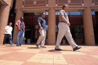
Figure 1. Gait

The study on the gait processing of an individual was initiated in the field of medicine to examine the walking patterns of impaired patients [1,2]. A decade after, it was first used as a pattern recognition technique by Johansson when he used reflectors affixed to the joints of a human body and showed motion sequences as the person walks[3]. The observers were able to identify gender and in some cases person recognition was obtained. Previous works on the use of gait for person identification have mostly utilized side-view gait (pendulum analogy) for feature extraction because temporal variations are more obvious from the side than the front. In this activity, we show and test the biometric feature developed by Soriano et al. that uses the idea of silhouette extraction, the freeman vector code and vector gradients to characterize the concavities and convexities in an image[4].

Experiment

Our first task was to capture an object against a steady background. In one of our conversations in class, Dr. Soriano suggested to use my mouth as the object mainly because she was curious if silhouette extraction can be applied to investigate the relationship between the opening of the mouth and the words (or sound) produced. If we are able to establish the said technique, then it could be a big help in the communication industry since communications with the use of web cameras nowadays is becoming widespread.

We then got the edge of the object of interest using edge detection algorithms and made sure that the edges were one-pixel thick. This is very important as problems may arise in the reconstruction of the curve spreads when the edges are more than a pixel thick. In fact, I encountered problems in the early part of the activity mainly because of the large size of my image and the edges, which were thicker than a pixel. To find the x-y coordinates of the edge, we used the regionprops and pixellist in Matlab.

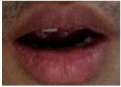
Figure 2. Sample mouth image (image size: 170 x 122)

Figure 3. Image after applying the edge detection algorithms which include: (a). im2bw (b) edge and bwmorph and imfill.

Note that all the neighboring pixels of an edge pixel can be represented by one number only (from 1 to 8) in the Freeman vector code as shown in Figure 4. We then replaced the edge pixel coordinates with their Freeman Vector Code, took the difference between the codes of two adjacent pixels and performed a running sum of three adjacent gradients. The vector gradient details include: concavity (negative values), convexity (positive numbers bounded by zeros) details and straight line (zeros).

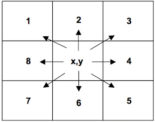
Figure 4. Freeman Vector Code illustration.

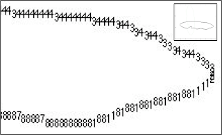
Figure 5. The pixel edges of the image with corresponding Freeman Vector code. Inset shows the whole Freeman vector code for the mouth image.

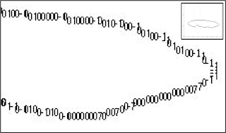
Figure 6. Processed image with corresponding values for the vector gradients. Inset shows the vector gradients for the mouth image.

Figure 6 shows the chain of zeros, positive and negative numbers placed in their appropriate pixel coordinates where zeros are regions of straight lines, negatives are regions of concavities and positives are regions of convexities.

Tips:

One of the more challenging steps in this activity is obtaining an image which is one-pixel thick after edge detection. Before my mouth, which was a success, I tried taking a picture of a hat, a watch and even my pen to no avail.

Since we were able to accurately reconstruct the different regions in the image, this activity may jumpstart the research in identifying the relationship between the shape of the mouth opening and the sound produced. I give myself a grade of 10 in this activity since I was able to reconstruct the regions of straight lines(zeros), concavities(negatives) and convexities(positives) placed in the appropriate pixel coordinates.

References:

[1] Murray, M.P., Drought, A.B., Kory, R.C. 1964. Walking Patterns of normal men. J. Bone Joint Surg. 46-A (2), 335-360.

[2] Murray, M.P 1967. Gait as a total pattern movement. Am. J. Phys. Med. 46(1), 290-232

[3] Johansson G., 1975. Visual Motion Perception. Sci. Am. 232, 76-88.

[4] Soriano, M., Araullo, S. and Saloma, C. 2004. Curve Spreads – A biometric from front-view gait video, Pattern Recognition Letters, 25, 1595-1602.

For teaching concerns please visit: https://sites.google.com/site/alongjas/

Activity 2: Hough Transform

I. Theory

The Hough Transform was patented by--surprise!--Paul Hough in 1960. The classic Hough transform was concerned with the identification of the lines in an image. It was later developed and popularized, two decades after, with its application to any arbitrary shape like circles and ellipses. It is now widely used in a variety of related methods for shape detection since it is tolerant of gaps in feature boundary descriptions and is relatively unaffected by image noise. This feature extraction technique is used in a wide range of fields including computer vision, image analysis and digital image processing.

II. Experiment

We were tasked to capture a gray scale image of a scene with straight lines. The image I chose was that of a lion inside a steel cage taken in the Baluarte mansion of then Ilocos Sur governor Chavit Singson. I had to first binarize the image (convert into its black and white version) and did edge detection before proceeding with the Hough transform technique. A successful implementation of this technique will result in an image with lines properly superimposed on straight edges in the image.

Figure 1. Image of a lion inside a cage taken in Balaurte, Ilocos Sur (image size: 450 x 600).


Figure 2. Black and white version of the sample lion image using the im2bw command in Matlab.
Figure 3. The edges in the lion image using the edge detection algorithm available in Matlab.

The Hough transform is designed to detect lines using the parametric representation of a line:

rho = x * cos(theta) + y * sin(theta) (1)

Rho is the distance from the origin to the line along a vector perpendicular to the line and theta is the angle between the x-axis and this vector.

We then used Hough Transform function in Matlab to create an accumulator matrix based on the parameters r and θ. Then we found the peaks in the accumulator matrix and converted the r and θ values into the equation of a line.

Figure 4. Computed Hough Transform of our image in 'hot' color map version with the peaks represented by the small squares

Figure 5. Superimposed lines on the original image indentified using the Hough Transform.


Figure 5 shows the superimposed lines on the cage, in the original image identified by the Hough Transform technique. The blue line represents the longest identified straight edge while the green lines represent the other straight edges. Comparing Figures 1 and 5, we notice that the Hough transform reconstructed the thin straight edges and those that easily blend with the background(faint ones).

Tips:

1. The hough function in Matlab easily generates a parameter space matrix whose rows and columns correspond to the rho and theta values respectively.

2. After computing for the Hough transform, use the houghpeaks function to find the peak values in the parameter space. The peaks represent potential lines in the input image

3. Use houghlines to find the endpoints of the line segments corresponding to the peaks in the Hough transform. The function automatically fills in gaps in the line segments.

We were successful in identifying the straight edges in our cage image by using the classic Hough transform. I give myself a grade of 10 in this activity. This activity is much easier than the first one, adaptive segmentation and tracking using the color locus, mainly because the functions needed are readily available in Matlab.


References:

[1] http://www.cogs.susx.ac.uk/users/davidy/teachvision/vision4.html

[2] Maricor Soriano, Applied Physics Lectures: Hough transform. 2009

[3] MATLAB R2008a

For teaching concerns please visit: https://sites.google.com/site/alongjas/